how to make negative numbers red in excel

Show Negative Numbers in Bracket and in Red Color. You can display negative numbers by using the minus sign parentheses or by applying a red color with or without parentheses.

How To Make Negative Numbers Red In Excel

How can I add this.

. When you are working with lots of different numbers in Excel you sometimes want your numbers to stand out by showing them in a negative red number enclosed in parenthesis. You can display negative numbers by using the minus sign parentheses or by applying a red color with or without parentheses. All of my spreadsheets display negative numbers in red rather than preceded by a negative sign. Go to the Home Tab.

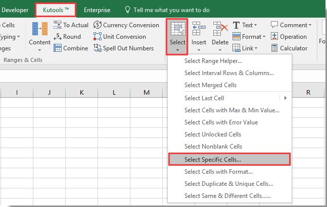
Format the cell value red if negative and green if positive with Format Cells function. If youre using Windows press Ctrl1. For example values below zero should stand out. The Select Specific Cells utility of Kutools for Excel helps you to select all cell with negative numbers at.

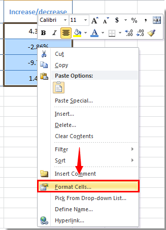
Hi I like to use the accounting format in excel. 1Select the list of cells that you want to use and then right click to choose Format Cells from the context menu see screenshot. Our guide continues below with another way to format negative numbers as red including pictures of those steps. A good Excel table provides a quick overview of the most important facts and figures.

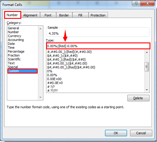
Right-click on a selected cell. The first option to make negative numbers red is to use a custom number format. Microsoft Excel How to Make Negative Numbers Red. However there is not an option to put negative numbers in red the currecny format can do this.

In the Category box click either Number or Currency. Automatically Format Negative Numbers Red in ExcelBy default negative numbers are not shown in a different colour by default in Excel. To do this you need to select your numbers and press CTRL1 to bring up the Format dialogue box. This tip explains the two ways you can format those percentages so they appear red just like you want.

Please see the steps below for details. Make all negative numbers in red with Kutools for Excel. Select the cells which contain that list of the numbers as shown in the screenshot below. In the Category box click either Number or Currency.

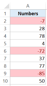
But for some reports negative numbers must be displayed with parenthesis. You will need to app. Say you have the list of numbers below in Column B and want to emphasize the negative numbers by making them red. Select the cell or range of cells that you want to format with a negative number style.

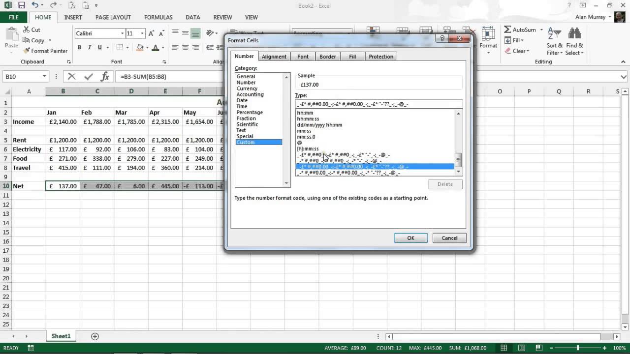
Select the cells to change. Select the Number tab in the Format Cells window then select Number in the category box. One format that isnt as easy to set up is for negative percentages. In Excel the basic way to format negative numbers is to use the Accounting number format.

The Format Cells function in Excel can help you to format the values as specific color based on the positive or negative numbers please do as this. In the Number group click on the Format Cell dialog box launcher. Mark negative numbers in red color can make users lookup negative numbers immediately by one glance so it is useful of us to learn how to make negative numbers red in worksheet. Select the cell or range of cells that you want to format with a negative number style.

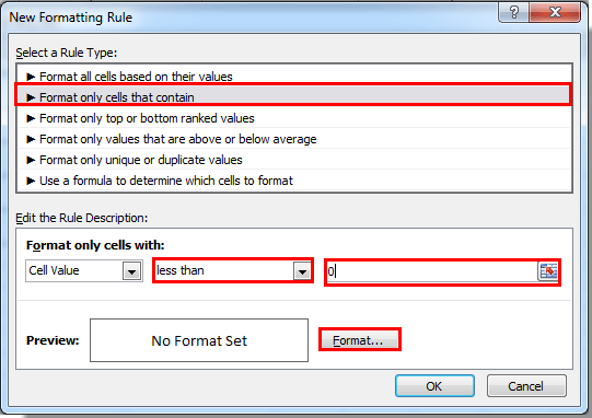
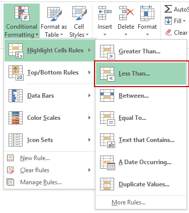
In this article well explore two ways of highlighting negative values in red color in Excel. You can find the dialog box launcher as a small square with an arrow inside it on the bottom. If youre using Windows press Ctrl1. Select the cell or range with numbers.

Negative numbers in Excel. Right click to bring up the dialog box from the list click Format Cells. Make Negative Numbers Red With a Custom Number Format. Lets see how to do that.

I want to retain all other characteristics of the format. Select the range of cells where you want negative numbers to be red and in the Ribbon go to. If youre using a Mac press 1. Click on the red numbers in the Negative Numbers box then click OK.

Click Number under Category. Excel includes quite a few different formats you can use for the information in a worksheet. I dont mind the red on the screen but when I print a worksheet those negative numbers come out a light gray because I use a black-and-white laser printer. Actually there are some tricks to make negative numbers red in excel this article will introduce you some of.

Open your Excel file. If youre using a Mac press 1. This option will display your negative number in red. In Excel you can turn negative numbers to red or add parentheses to make them much easier to read.

If you have applied a specific format to your cells such as Currency Accounting Percentage Fraction Scientific or Special select that category instead of Number. One way of highlighting important numbers is by using colors. Select a red number under Negative numbers then click OK.

How To Make All Negative Numbers In Red In Excel